Imagine we have different ways to write the same code. How do we figure out which one is the best? That's where Big O notation comes in. It helps us measure how much time and space the code will need, making it easier to compare them.

What is Big-O Notation?

Big O, also known as "Order of," is a way to describe how long an algorithm might take to run in the worst-case scenario. It gives us an idea of the maximum time an algorithm will need based on the input size. We write it as O(f(n)), where f(n) shows how many steps the algorithm takes to solve a problem with input size n.

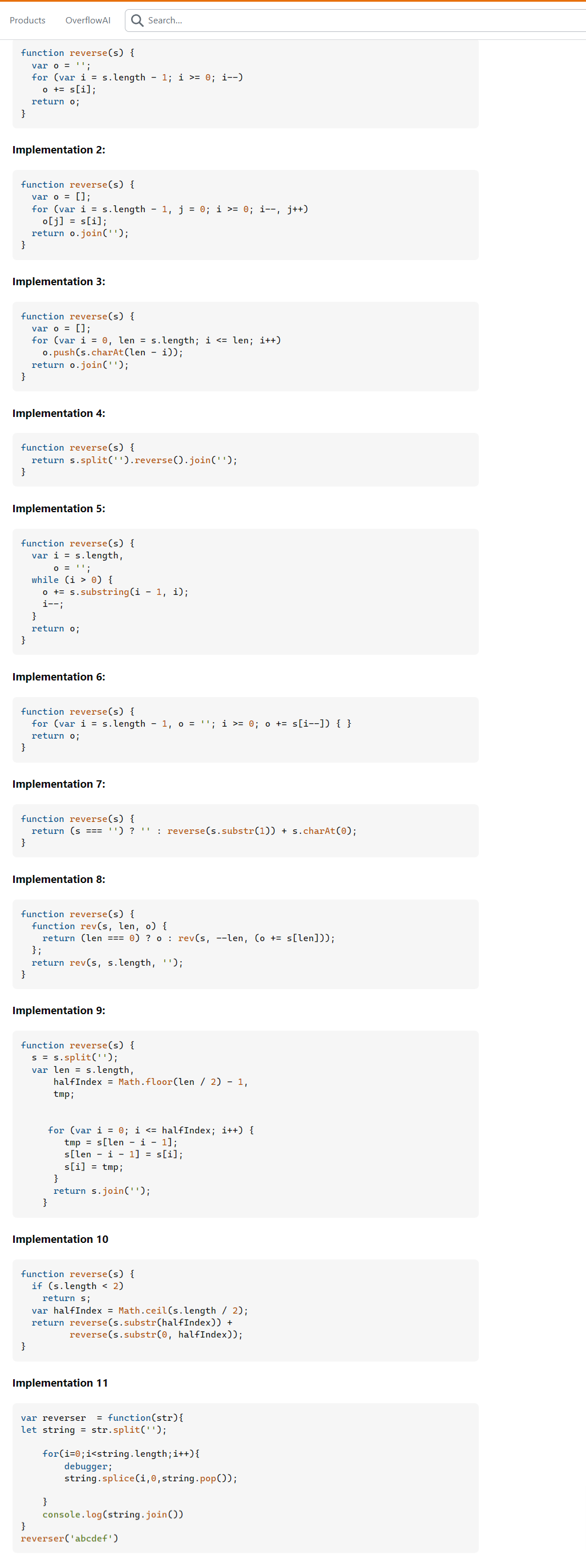
Let’s try to understand by an example “Write a function that accepts a string input and returns a reversed copy“

Alright, I'm sharing a Stack Overflow solution with you, along with the image above, as you can see. It shows 10 different ways to solve the same problem, each with a unique approach.

Now, the question is: how do we know which one is the best?

Our goal is to understand time and space complexity. To do this, let's explore a concrete example with two different code snippets, so we can clearly see how these concepts matter.

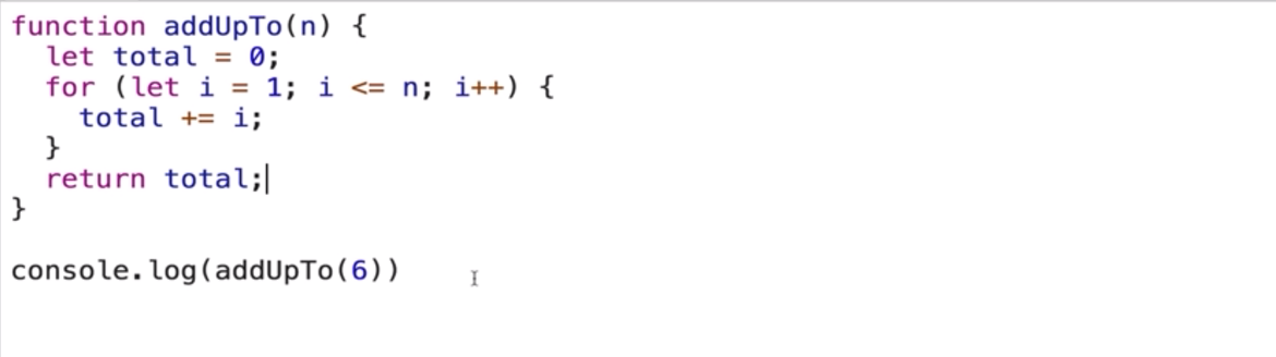
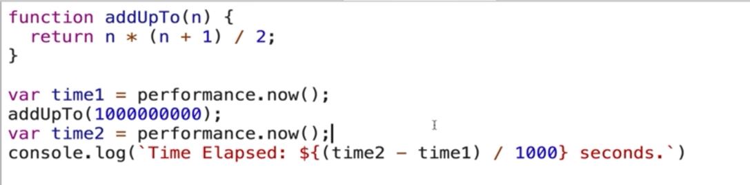
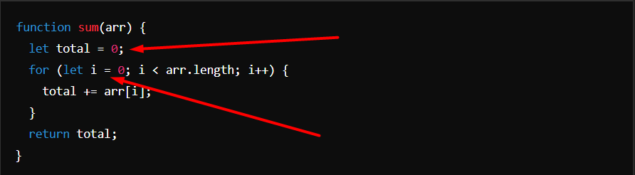
Here's a function called addUpTo. This function uses a for loop that runs until it reaches the length of n and returns the total sum.

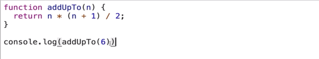
Now, let's look at another example that achieves the same functionality:

Which one is better?

Now, what does 'better' really mean in this context?

• Is it faster?

• Does it use less memory?

• Is it more readable?

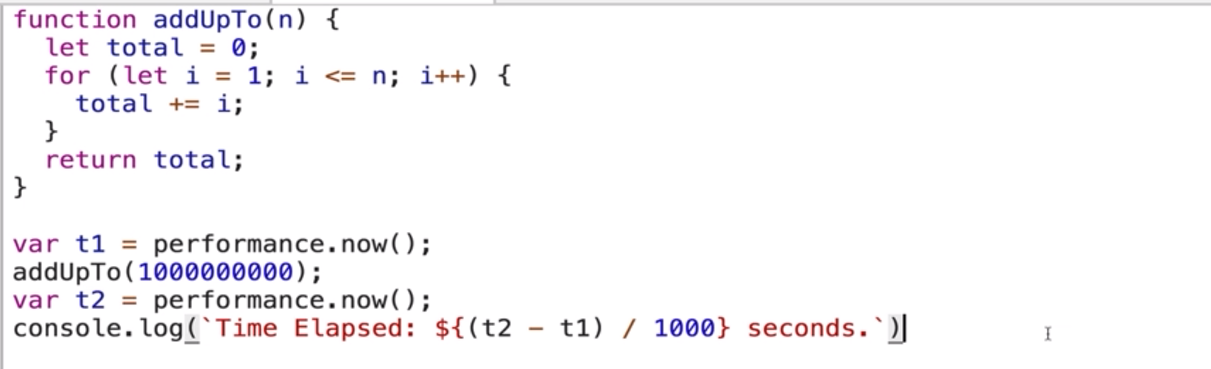
Typically, people focus on the first two—speed and memory usage—before considering readability. In this case, we'll be focusing on the first two. To measure the performance of both code examples, we'll use JavaScript's built-in timing functions to analyze and compare their execution times.

In the code above, I've added t1 and t2, which utilizes the performance.now() function built into JavaScript. This function helps us measure the time taken by the code to execute, allowing us to accurately compare the performance of the two approaches.

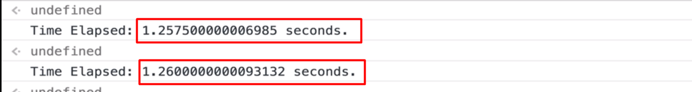
Exactly, the execution time varies depending on different factors, and you can see that on my computer as well—the times aren't consistent. The performance.now() function doesn't give us a fixed time, but it provides a useful estimate for comparison.

Now, let's take a look at the second example:

Now, observe the difference in execution time between the first and second code examples. The second one is noticeably faster than the first.

But what's the issue with relying solely on time measurements?

• Different machines record different times.

• Even the same machine will record different times on each run.

• For very fast algorithms, speed measurements may not be precise enough to give an accurate comparison.

These factors make time-based performance assessments unreliable, especially for quick algorithms.

Okay, if not time then what?

That’s where Big O will help us to measure the time complexity and space both. So Big O Notation is a way to formalize fuzzy counting. It allows us to talk formally about how the runtime of algorithm grows as the input grows.

We say that an algorithm is O(f(n)) if the number of simple operations the computer has to do is eventually less than a constant times f(n), as n increases.

• f(n) could be linear (f(n) = n)

• f(n) could be quadratic (f(n) = n2)

• f(n) could be constant (f(n) = 1)

• f(n) could be something entirely different!

Here is an example:

In this case, we only have 3 operations, and no matter the size of the input, it will always remain 3 operations. This is why we can say that the time complexity of this function is constant, or O(1).

Now here is the first example:

In this case, as the input n grows, the number of operations also increases proportionally. Therefore, the time complexity depends on the size of the input, making it O(n).

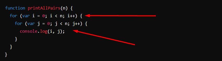
Now, let's look at another example:

In this example, we have two nested for loops, both dependent on n—the input. This means that as the input n grows, the number of operations increases significantly. As a result, the time complexity of this code is O(n²), also known as quadratic time complexity.

Now, let's simplify Big O Notation. When determining the time complexity of an algorithm, there are a few helpful rules of thumb to keep in mind. These guidelines arise from the formal definition of Big O notation and make it easier to analyze algorithms.

Constants don’t matter

• O(2n) = O(n)

• O(500) = O(1)

• O(13n²) = O(n²)

• O(n+ 10) = O(n)

• O(1000n + 500) = O(n)

• O(n² + 5n + 8) = O(n²)

Big O Shorthands

1. Arithmetic operations are constant

2. Variable assignment is constant

3. Accessing elements in an array (by index) or object (by key) is constant

4. In a loop, the complexity is the length of the loop times the complexity of whatever happens inside the loop

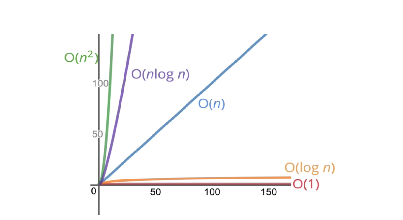
Here is the Big O Chart:

So far, from the examples, we've learned about O(n) (linear time complexity), O(1) (constant time complexity), and O(n²) (quadratic time complexity). These cover the basic patterns where operations grow with input size.

We'll discuss O(log n) and O(n log n)—logarithmic and linearithmic time complexities—a bit later.

Space Complexity

So far, we've been focusing on time complexity: how can we analyze the runtime of an algorithm as the size of the inputs increases?

We can also use big O notation to analyze space complexity: how much additional memory do we need to allocate in order to run the code in our algorithm?

What about the inputs?

Sometimes you'll hear the term auxiliary space complexity to refer to space required by the algorithm, not including space taken up by the inputs. Unless otherwise noted, when we talk about space complexity, technically we'll be talking about auxiliary space complexity.

Space Complexity in JS

• Most primitives (booleans, numbers, undefined, null) are constant space

• Strings require O(n) space (where n is the string length) Reference types are generally O(n), where n is the length (for arrays) or the number of keys (for objects)

Remember, we're talking about space complexity, not time complexity. In this code, we can see we only have two variables. No matter how large the input grows, these two variables will always exist in the code. Since we're not adding any new variables as the input increases, we can say that the space complexity is O(1), meaning it's constant space complexity.

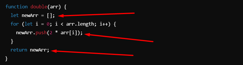
Let’s understand with another example:

In this code, the function returns newArr after doubling every element in the input array. Since the size of newArr is directly proportional to the size of the input arr, the space used by newArr grows with the input size. Unlike the previous example, where space was constant, here the space complexity depends on the size of the input array. Therefore, the space complexity is O(n), meaning it's linear.

I hope this makes space complexity clearer—just like time complexity, we're measuring it using Big O notation. So far, you've learned about different time complexities, in increasing order of complexity: O(1), O(log n), O(n), O(n log n), O(n²), O(n³), and so on. However, we haven't yet explored logarithmic time complexity.

Next, we'll dive into logarithmic time complexity and see how it works.

Logarithms

We've encountered some of the most common complexities: O(1), O(n), O(n2). Sometimes big O expressions involve more complex mathematical expressions. One that appears more often than you might like is the logarithm!

What's a log again?

log2 (8) = 3 → 2³ = 8

log2 (value) = exponent → 2^exponent = value

We'll omit the 2, which means:

log === log2

The logarithm of a number roughly measures how many times you can divide that number by 2 before it becomes less than or equal to 1. This makes logarithmic time complexity very efficient. As you saw in the chart, O(1) (constant time) is very close to O(log n), which is fantastic! It's also worth noting that O(n log n) is much better than O(n²) in terms of efficiency, making it a preferred complexity for many algorithms.

• Certain searching algorithms have logarithmic time complexity.

• Efficient sorting algorithms involve logarithms.

• Recursion sometimes involves logarithmic space complexity.

Great! We've covered most of the key points on space and time complexity. Keep in mind that mastering these concepts takes practice, so don't feel overwhelmed if it's not completely clear right away. Take your time, review the material multiple times, and revisit examples as needed. It often takes a few repetitions for these ideas to really sink in, so be patient with yourself!

Finally, let’s do one more time recap:

• To analyze the performance of an algorithm, we use Big O Notation

• Big O Notation can give us a high-level understanding of the time or space complexity of an algorithm

• Big O Notation doesn't care about precision, only about general trends (linear? quadratic? constant?)

Again, Big O Notation is everywhere, so get lots of practice!

---

We at CreoWis believe in sharing knowledge publicly to help the developer community grow. Let’s collaborate, ideate, and craft passion to deliver awe-inspiring product experiences to the world.

Let's connect:

• X/Twitter

• LinkedIn

• Website

This article is crafted by Syket Bhattachergee, a passionate developer at CreoWis. You can reach out to him on X/Twitter, LinkedIn, and follow his work on the GitHub.